GeoDataViewer Studio now includes spatial analysis tools. You can create buffers, measure features, generate new geometry, and compare polygon layers in the same workspace where you view your data.
Select a layer, open Spatial analysis, and choose an operation. The result appears as a new layer alongside the source. You can change its style, inspect its attributes, or use it in another analysis.
The calculations run locally in your browser. Files you open from your device are not uploaded for analysis; remote sample datasets and basemaps still need network access.
Open Studio and try spatial analysis →
Create buffers around your features
A buffer turns a distance into an area on the map. A point becomes a circular polygon, a line becomes a corridor, and a polygon expands outward. A negative distance can shrink a polygon inward.
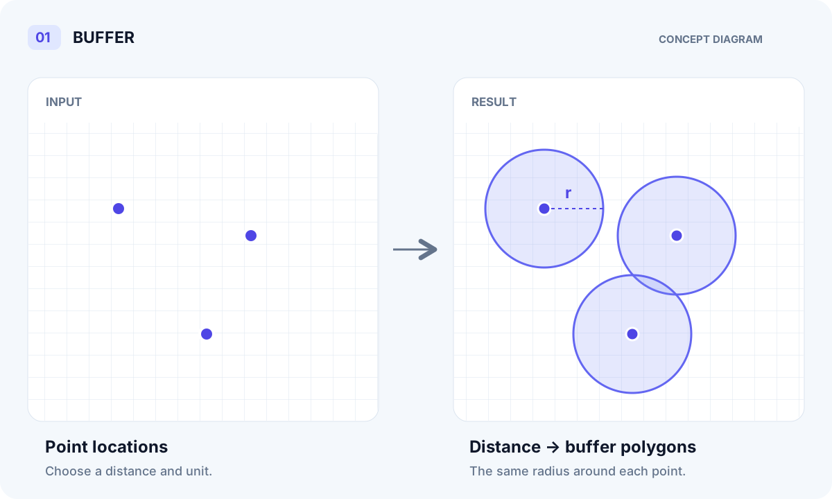
To try it with the built-in city sample:
- Open Sample Data in Studio and add US Cities to the map.
- Select the US Cities layer, then open Spatial analysis.
- Set a buffer distance and choose kilometers, meters, miles, nautical miles, or feet. Try 100 kilometers to make the result easy to see at a national scale.
- Click Buffer features. A new polygon layer appears in the layer list.
- Give the result a different color from the city markers, and zoom in to compare them.
Enable Merge overlapping buffers if you want connected buffer areas combined. Separate areas remain separate shapes. This is useful when exploring proximity around several sites or a corridor along a route.
The unit matters: a 1-kilometer buffer is small when the map shows an entire country. If a result is hard to see, zoom closer before increasing the distance. A buffer measures geographic distance; it does not model roads, traffic, or walking routes.
Create centroids from lines and polygons
Centroids creates one point for each input line or polygon feature. The points retain the source attributes, so you can style them by a field or inspect them in the attribute table.
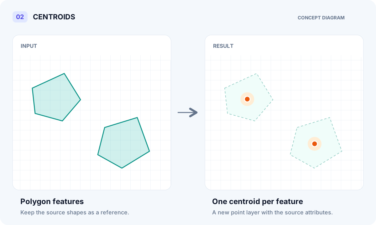
For a simple example, add World Lakes from Sample Data, select its polygon layer, and click Centroids. Keep the lakes and the new points visible together, then give the points a contrasting color.
The tool uses the mean of the geometry’s vertices. It is not an area-weighted center of mass, and a centroid is not guaranteed to lie inside a concave polygon or one part of a multipart feature. Use it as a geometric summary rather than an automatically valid site location.
Compare two polygon layers
The Overlay section contains two operations:
- Intersect keeps the area shared by both polygon layers.
- Difference removes the second layer’s area from the active layer.
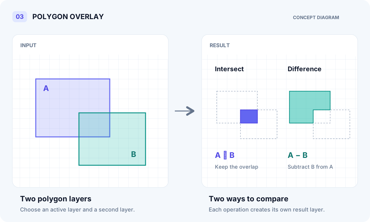
To explore this workflow:
- Load two polygon datasets. World Land and World Lakes are available in Sample Data.
- Select World Land as the active layer.
- Open Spatial analysis and choose World Lakes in the Overlay layer dropdown.
- Click Intersect to create the shared areas, or Difference to subtract the lakes from the land polygons.
- Hide the input layers temporarily to inspect the result on its own.
Both inputs need polygon geometry. An intersection can correctly return no features when the layers do not overlap. A difference can also be empty when the second layer covers the first completely. The results depend on the boundaries in your input data, including their resolution and any existing holes.
After an operation, Studio selects the new result layer. Select the original layer again if you want to run a different operation on the same input.
More tools in the same panel
The launch includes eight operations:
| Tool | What it produces | Example use |
|---|---|---|
| Buffer | Polygons at a chosen distance from features | Explore proximity around cities or rivers |
| Add area / length columns | area_km2 for polygons and length_km for lines | Compare lake areas or river lengths |
| Centroids | A point for each line or polygon feature | Create a point representation of shapes |
| Bounding boxes | An axis-aligned bounding polygon for each feature | Compare the spatial spread of lines or polygons |
| Layer extent | One bounding polygon for the whole layer | See a dataset’s overall coverage |
| Dissolve | Merged polygon geometry, optionally grouped by an attribute | Combine touching or overlapping areas |
| Intersect | The shared areas of two polygon layers | Find overlapping coverage |
| Difference | The part of the active polygon layer outside the second | Remove an exclusion area |
For measurements, open the result layer’s Attribute Table to see the new columns. Areas and lengths are geodesic measurements based on WGS84, expressed in square kilometers and kilometers respectively.
For Dissolve, choose a grouping field to merge polygons within each attribute group, or leave it unset to process the layer together. Disconnected pieces can remain separate output features; a group does not necessarily become a single connected shape.
Bounding boxes are most useful for shapes with a nonzero width and height. A single point has a zero-area box, so buffering is the better choice when you want a visible area around point locations.
A few practical tips
- Start with clean geometry and a small dataset. Large or complex layers can take longer to process in the browser. Check unexpected results against the source data.
- Use contrasting styles. A source layer and a result with the same color can be difficult to distinguish. Toggle visibility to compare them.
- Check your active layer. The panel names the layer being analyzed, and a successful operation makes its result active.
- Read the attributes as well as the map. Measurement columns and copied source fields help explain what a result represents.
These tools are designed for quick exploration: open data, test a spatial relationship, and inspect the result without leaving the browser.
Try the new spatial analysis tools in Studio →
Looking for something to analyze? Browse the dataset catalog or start with the Natural Earth country boundaries.