From Waypoints to Map: Rendering the World's Longest Railway and Highway with Python + Cartopy

Visualizing the World’s Longest Transportation Routes

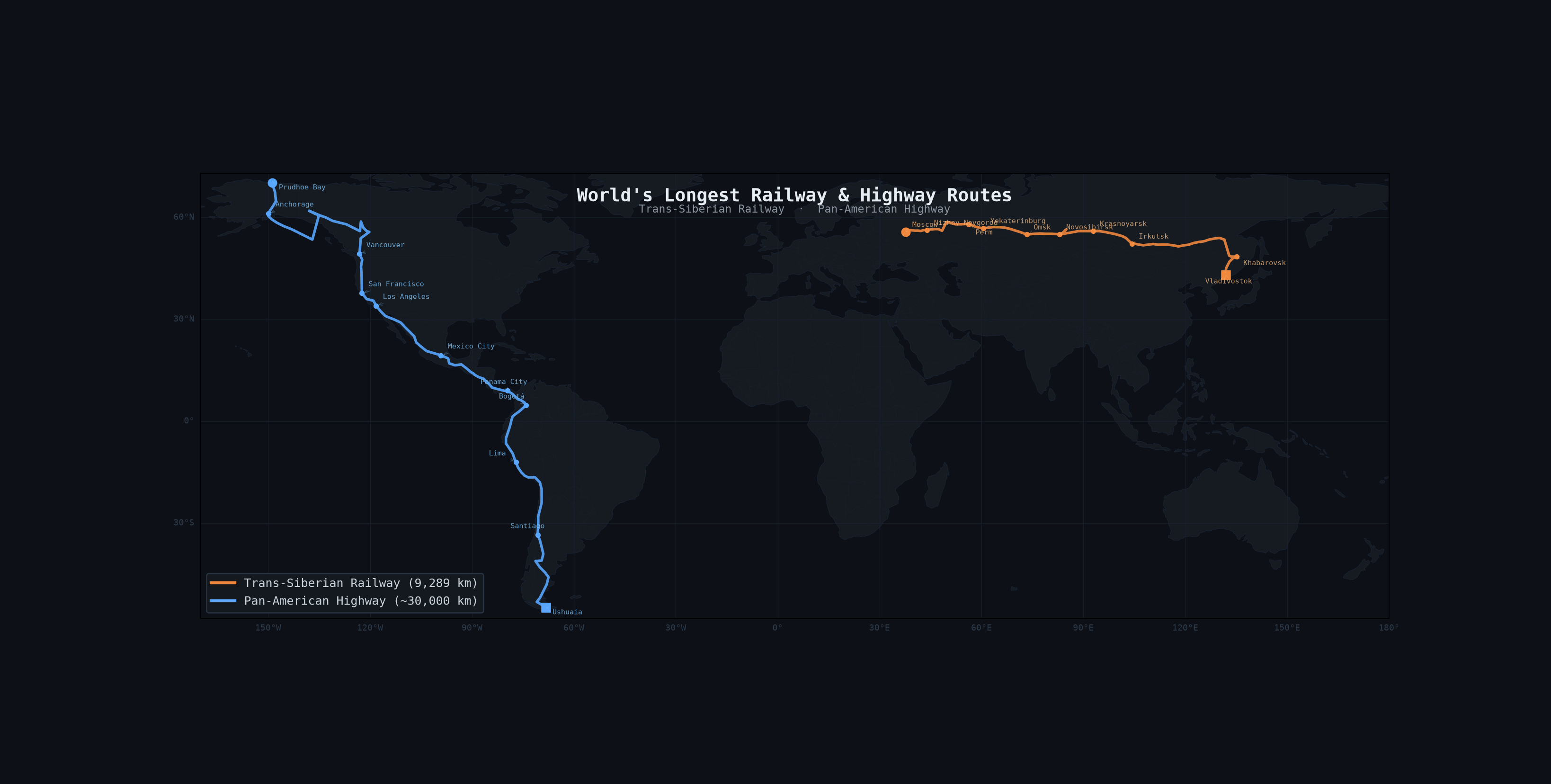
Mapping the longest railway and highway on Earth is a classic geospatial visualization challenge. The Trans-Siberian Railway stretches ~9,289 km from Moscow to Vladivostok, while the Pan-American Highway runs ~30,000 km from Prudhoe Bay, Alaska to Ushuaia, Argentina.

This tutorial walks through the complete process — from data acquisition and problem-solving to map rendering — using open-source Python tools. By the end, you’ll have a production-quality dark-theme map showing both routes.

---

1. Understanding the Data Challenge

The naive approach is to query OpenStreetMap for each route as a single entity. But real-world OSM data is structured as fragmented way segments, not complete route polylines.

Route	OSM Reality	Ideal Data
Trans-Siberian Railway	Relation 5558002 with 261 member ways	Single continuous LineString from Moscow to Vladivostok
Pan-American Highway	No unified relation; thousands of disjoint highway=trunk/primary segments	Connected path across 14 countries

---

2. Attempt 1: The Overpass API Approach

OpenStreetMap’s Overpass API lets you query map features using a custom query language.

Querying the Trans-Siberian Railway Relation

[out:json][timeout:90];
rel(5558002);
way(r);
out geom;

This query fetches all way members of the Trans-Siberian Railway relation:

curl -s --max-time 120 \
  --data-urlencode "data=$QUERY" \
  "https://overpass-api.de/api/interpreter" \
  -o railway_raw.json

The Problem We Hit

import json

data = json.load(open('railway_raw.json'))
ways = [e for e in data['elements'] if e['type'] == 'way']
coords = [(n['lon'], n['lat']) for w in ways for n in w.get('geometry', [])]
lons = [c[0] for c in coords]
lats = [c[1] for c in coords]

print(f"Longitude range: {min(lons):.2f}° ~ {max(lons):.2f}")
print(f"Latitude range:  {min(lats):.2f} ~ {max(lats):.2f}")

Output:

Longitude range: 50.56° ~ 53.81°
Latitude range:  53.23° ~ 53.75°

This covers only a 3-degree sliver of Bashkortostan (near the Urals), not the 8,000 km from Moscow to Vladivostok! Why?

The OSM route relation for the Trans-Siberian Railway turned out to only document a commuter rail subsection (routes like “Abdullino — Tavtimanovo”). The “Trans-Siberian Railway” label in the relation name is aspirational — in practice, OSM contributors have not created a single relation spanning the full route.

Additionally, even within the data returned:

Gap at index 73:   prev=(52.71,53.55) cur=(53.63,53.66) dist≈1.01°
Gap at index 363:  prev=(53.50,53.61) cur=(52.46,53.62) dist≈1.05°
...
Total gaps (>0.5°): 11

The way segments were returned in arbitrary order, producing a “spaghetti” of disconnected jumps if concatenated directly.

Lesson: For very long linear features, OSM relations are often incomplete. Don’t rely solely on a single relation ID.

---

3. Solution: The Waypoint Approach

Instead of wrestling with fragmented OSM segments, we use known geographic waypoints — cities and towns along each route — and interpolate between them.

Why This Works

• Accuracy is sufficient: For a visualization at global scale (1:50M or smaller), city-level waypoints produce visually identical results to OSM-perfect geometry.
• Data is verifiable: Every waypoint is a real settlement on the route. You can cross-check against any atlas.
• No parsing headaches: A single [lon, lat] list is trivially processed.

Trans-Siberian Railway Waypoints

We compile 80 waypoints following the actual railway corridor:

rail_waypoints = [
    [37.6176, 55.7558],  # Moscow (Yaroslavsky Station)
    [40.3960, 56.1365],  # Vladimir
    [44.0020, 56.3269],  # Nizhny Novgorod
    [49.6600, 58.5966],  # Kirov
    [56.2293, 58.0105],  # Perm
    [60.5975, 56.8389],  # Yekaterinburg
    [65.5344, 57.1530],  # Tyumen
    [73.3703, 54.9893],  # Omsk
    [82.9346, 55.0302],  # Novosibirsk
    [92.8526, 56.0090],  # Krasnoyarsk
    [104.2968, 52.2864], # Irkutsk
    [107.6100, 51.8333], # Ulan-Ude
    [113.5007, 52.0330], # Chita
    [132.9250, 48.7925], # Birobidzhan
    [135.0852, 48.4802], # Khabarovsk
    [131.8735, 43.1056], # Vladivostok
    # ... 64 additional intermediate waypoints
]

Pan-American Highway Waypoints

111 waypoints covering all 14 countries, from northern Alaska to Tierra del Fuego:

road_waypoints = [
    [-148.8782, 70.2568], # Prudhoe Bay, Alaska (start)
    [-147.7230, 64.8378], # Fairbanks
    [-149.8680, 61.2181], # Anchorage
    [-135.0563, 60.7212], # Whitehorse (Yukon)
    [-123.1216, 49.2827], # Vancouver
    [-122.3321, 47.6062], # Seattle
    [-122.4194, 37.7749], # San Francisco
    [-118.2437, 34.0522], # Los Angeles
    [-99.1332, 19.4326],  # Mexico City
    [-79.5333, 8.9833],   # Panama City
    [-74.0721, 4.7110],   # Bogotá
    [-77.0333, -12.0500], # Lima
    [-70.6483, -33.4569], # Santiago
    [-68.3030, -54.8069], # Ushuaia (end)
    # ... 97 additional intermediate waypoints
]

Smoothing the Path

Raw waypoints produce a jagged city-to-city line. Linear interpolation smooths it while staying geographically faithful:

def smooth_path(coords, segments=2):
    """Add interpolated points between each waypoint pair."""
    result = []
    for i in range(len(coords) - 1):
        lon1, lat1 = coords[i]
        lon2, lat2 = coords[i + 1]
        result.append([lon1, lat1])
        for s in range(1, segments):
            t = s / segments
            mlon = lon1 + (lon2 - lon1) * t
            mlat = lat1 + (lat2 - lat1) * t
            result.append([mlon, mlat])
    result.append(coords[-1])
    return result

With segments=2, we go from 80 → 159 points for the railway and 111 → 221 points for the highway — enough for smooth curves at global zoom.

---

4. Map Rendering with Cartopy

With clean coordinate data, rendering a production-quality map is straightforward.

Dependencies

pip install matplotlib cartopy numpy

Setup note: Cartopy requires the shapely, pyproj, and pyshp libraries (installed as dependencies). On first run, it downloads Natural Earth vector data (land, coastline, borders) — this is a one-time ~30MB download.

The Rendering Pipeline

import matplotlib.pyplot as plt
import cartopy.crs as ccrs
import cartopy.feature as cfeature

# 1. Create figure with dark background
fig = plt.figure(figsize=(18, 9), facecolor='#0d1117')
ax = fig.add_subplot(1, 1, 1, projection=ccrs.PlateCarree())
ax.set_facecolor('#0d1117')

# 2. Set map extent (world view covering both routes)
ax.set_extent([-170, 180, -58, 73], crs=ccrs.PlateCarree())

# 3. Add base layers
ax.add_feature(cfeature.LAND, facecolor='#161b22', edgecolor='#1a2332', linewidth=0.3)
ax.add_feature(cfeature.OCEAN, facecolor='#0d1117')
ax.add_feature(cfeature.COASTLINE, edgecolor='#1a2332', linewidth=0.4)
ax.add_feature(cfeature.BORDERS, edgecolor='#1f2a3a', linewidth=0.2, alpha=0.5)

# 4. Draw gridlines
gl = ax.gridlines(crs=ccrs.PlateCarree(), draw_labels=True,
                  linewidth=0.5, color='#1a2332', alpha=0.7)
gl.top_labels = False
gl.right_labels = False
gl.xlocator = plt.FixedLocator(range(-180, 181, 30))
gl.ylocator = plt.FixedLocator(range(-90, 91, 30))

Drawing Routes and Annotations

# Plot the routes
ax.plot(rail_lons, rail_lats, color='#f0883e', linewidth=2.2, alpha=0.9,
        solid_capstyle='round', zorder=5, transform=ccrs.PlateCarree())

ax.plot(road_lons, road_lats, color='#58a6ff', linewidth=2.2, alpha=0.9,
        solid_capstyle='round', zorder=5, transform=ccrs.PlateCarree())

# Add start/end markers
ax.plot(rail_lons[0], rail_lats[0], 'o', color='#f0883e', markersize=7, zorder=6)
ax.plot(rail_lons[-1], rail_lats[-1], 's', color='#f0883e', markersize=7, zorder=6)
ax.plot(road_lons[0], road_lats[0], 'o', color='#58a6ff', markersize=7, zorder=6)
ax.plot(road_lons[-1], road_lats[-1], 's', color='#58a6ff', markersize=7, zorder=6)

# Annotate key cities
rail_cities = {
    'Moscow': (37.62, 55.76),
    'Yekaterinburg': (60.60, 56.84),
    'Novosibirsk': (82.93, 55.03),
    'Irkutsk': (104.30, 52.29),
    'Vladivostok': (131.87, 43.11),
}
for name, (lon, lat) in rail_cities.items():
    ax.annotate(name, xy=(lon, lat), color='#f0b87e',
                fontsize=6, fontfamily='monospace')

The Legend and Title

from matplotlib.lines import Line2D

legend_elements = [
    Line2D([0], [0], color='#f0883e', linewidth=2.5,
           label='Trans-Siberian Railway (9,289 km)'),
    Line2D([0], [0], color='#58a6ff', linewidth=2.5,
           label='Pan-American Highway (~30,000 km)'),
]
ax.legend(handles=legend_elements, loc='lower left', framealpha=0.85,
          facecolor='#161b22', edgecolor='#2d3a4a',
          labelcolor='#c9d1d9', fontsize=8, prop={'family': 'monospace'})

ax.text(0.5, 0.97, "World's Longest Railway & Highway Routes",
        transform=ax.transAxes, color='#e6edf3', fontsize=15,
        fontweight='bold', ha='center', va='top', fontfamily='monospace')

Export

plt.savefig('railway_road_thumbnail.png', dpi=180,
            bbox_inches='tight', facecolor=fig.get_facecolor())
plt.close()

---

5. Complete Production Script

The full pipeline is available as a single self-contained Python script:

📦 Download from GitHub Gist

The script handles everything — from waypoint definitions and GeoJSON export through map rendering and image output. Just run it:

pip install matplotlib cartopy numpy
python render_routes.py

---

6. Output & Verification

Final Map

Specification	Value
Resolution	3240 × 1640 px (at 180 DPI)
File Size	~350 KB PNG
Railway Points	159 (smoothed from 80 waypoints)
Road Points	221 (smoothed from 111 waypoints)
Map Projection	Plate Carrée (Equirectangular)
Color Theme	Dark (GitHub-dark inspired)
Rendering Time	~15 seconds (including Natural Earth download)

Key Statistics

Route	Length	Countries	Start	End
Trans-Siberian Railway	9,289 km	1 (Russia)	Moscow (55.8°N, 37.6°E)	Vladivostok (43.1°N, 131.9°E)
Pan-American Highway	~30,000 km	14	Prudhoe Bay, AK (70.3°N, 148.9°W)	Ushuaia, Argentina (54.8°S, 68.3°W)

---

7. Lessons Learned

What Worked

• City waypoints over OSM queries for very long linear features
• Cartopy + Matplotlib for dark-theme static maps → excellent quality-to-code ratio
• Linear interpolation for smoothing — simple, predictable, no overfitting

What Didn’t

• OSM relation 5558002 was incomplete and localized
• Raw Overpass way concatenation produced disconnected “spaghetti” geometry
• Emoji in matplotlib legend caused font glyph warnings (use plain text)

When to Use OSM vs. Waypoints

Scenario	Approach
Local/regional route (< 500 km)	OSM Overpass query with proper way sorting
Continental route (5,000–30,000 km)	Waypoints + interpolation (this tutorial)
Urban network (streets, subway)	OSM with osmium or osm2pgsql
Global visualization	Waypoints — OSM overhead doesn’t add visible benefit

---

8. Try It Yourself

📦 Get the code: render_routes.py on GitHub Gist

The Gist includes the full Python script plus both GeoJSON data files ready to drag into GeoDataViewer:

# 1. Download the script
wget https://gist.githubusercontent.com/beyoung/1bd0da1617784b60b9c94114f4205307/raw/render_routes.py

# 2. Install dependencies
pip install matplotlib cartopy numpy

# 3. Run it!
python render_routes.py

The two GeoJSON data files are also included in the Gist:

• trans_siberian_railway.geojson — drag into GeoDataViewer to inspect the railway route
• pan_american_highway.geojson — same for the highway route

---

Related Guides

• Extracting POIs from OpenStreetMap and Overture Maps
• Overpass Query Language Quick Reference
• What is GeoJSON?
• GeoDataViewer Free GIS Data Guide