What we learned when a user tried to load a massive GML file in a browser.

---

The Problem That Started This

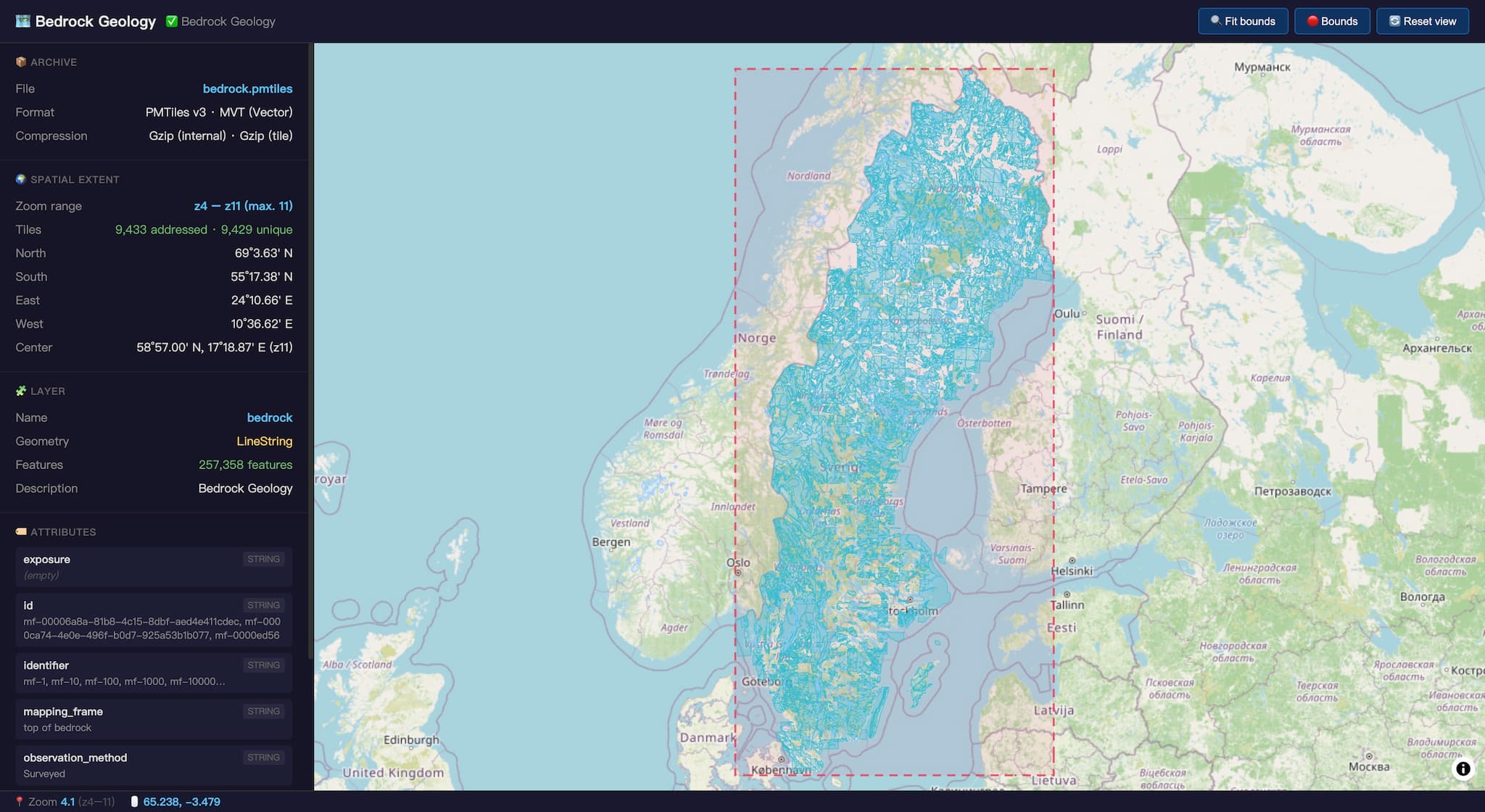
A few weeks ago, a GeoDataViewer user wrote in asking why a large GML file wouldn’t load in their browser. The file — a geological map from a national survey — was roughly 1 GB in size and contained hundreds of thousands of mapped features. They had downloaded open data, unzipped it, dragged it into a web map, and nothing happened.

This is not a bug report. This is a format problem.

And it’s a problem far bigger than this one user. Every day, GIS professionals, geological surveyors, urban planners, and hobbyists hit the same wall: they acquire perfectly good open data, try to view it in a modern web browser, and the browser just … gives up.

The solution exists. It has existed for over a decade. But most end users have never heard of it. This post is about why vector tiles are the answer, why partial solutions fall short, and why the gap between “it works in my desktop GIS” and “it works in my browser” remains the industry’s most underappreciated UX problem.

---

Part I: Why Browsers Can’t Handle Large Vector Datasets

The browser is not QGIS. It is not ArcGIS Pro. It is a sandboxed runtime with a strict memory budget, a single-threaded (ish) DOM, and no access to your disk.

Here is what happens when you drag a ~1 GB GML file into a web map:

Step 1: Memory saturation

The browser must read the entire file into memory. GML — like all XML-derived formats — is notoriously verbose. A ~1 GB GML file decompresses to roughly a gigabyte of XML text. Parse that into a DOM tree, and you are looking at 3–5 GB of peak memory for a naive parser. Even a streaming parser that outputs GeoJSON must materialize that data into an in-memory data structure. The resulting GeoJSON still requires the browser to hold the full dataset in memory before rendering can begin.

Chrome on a typical laptop with 8 GB of RAM will crash, swap to death, or throw an Out of Memory error.

Step 2: Parsing bottleneck

XML parsing in JavaScript is slow. DOMParser is not optimized for multi-hundred-megabyte documents. The browser’s main thread blocks for tens of seconds — or minutes — while it tries to build a document tree. There is no yield, no progress bar, just a frozen tab and a spinning cursor.

Step 3: Rendering collapse

Even if you somehow get the data into memory as GeoJSON, rendering hundreds of thousands of features is itself a challenge. Every feature becomes a DOM element in the canvas rendering pipeline. Every pan or zoom re-evaluates visibility, reprojects coordinates (if you forgot to pre-reproject — a second blocking operation), and redraws. Without tiling, the renderer must consider every feature on every frame. Frame rate drops below 1 FPS. The user gives up.

Why This Affects Every Flat Format

This is not a GML problem. It is a problem with every non-tiled vector format:

Format	Browser Issue	Memory for large datasets
GML	XML parsing is slow and memory-hungry; no native browser support	~3–5 GB (DOM)
Shapefile (.shp)	Requires binary parser; must be fully loaded before rendering	~600 MB–1 GB (uncompressed)
GeoJSON	De facto standard, but no streaming; entire file must parse before first draw	~700 MB+
GeoJSON Lines (.geojsonl)	Streamable line-by-line, but still must be held in memory as a single layer	~700 MB (reduced peak during load)
GeoParquet	Columnar, efficient for analytics; requires WASM or DuckDB in browser; no native rendering support	Depends on query — better, but needs complex tooling

Every single one of these formats shares the same fundamental limitation: the client must load the full dataset before it can render anything.

”But Desktop GIS Can Handle It” — No, It Can’t

A common reaction at this point is: “Well, browsers are weak. I’ll just use QGIS or ArcGIS — they’re built for this.”

The uncomfortable truth: they struggle too.

Loading a ~1 GB GML file into QGIS can take 5–10 minutes on a modern laptop. During that time, the application is frozen — no pan, no zoom, no attribute table, no progress bar beyond a vague “Loading…” in the status bar. ArcGIS Pro fares better on feature count, but its memory footprint for hundreds of thousands of features with full geometry sits at 1.5–2.5 GB — and that is before you open the attribute table, apply a symbology classification, or try to export a map. If your machine has 8 GB of RAM, you are now in swap territory.

This is not a browser-vs-desktop issue. It is a data model issue. When a format requires loading all geometry into memory before any operation — whether that operation is “render to screen” or “run a spatial query” — the bottleneck is the same. Desktop GIS has a larger budget (more RAM, direct disk access, native threading), but it does not have a different architecture. The full dataset still lands in memory.

The difference is degrees. A desktop application might take 5 minutes instead of crashing. But the user is still waiting. And the moment they need to share that data with a colleague on the web, they hit the browser wall anyway.

---

Part II: The Vector Tile Solution

Vector tiles break this cycle with a deceptively simple insight: don’t load everything. Load only what’s visible at the current zoom level.

A vector tile is a pre-tiled, pre-clipped chunk of data — typically 256×256 or 512×512 pixels at a given zoom level — encoded in a compact binary format (Mapbox Vector Tile / MVT, PBF). The browser requests tiles on demand as the user pans and zooms. Each tile is typically 10–100 KB. A session that views a national dataset may fetch only a few hundred tiles — a few megabytes total — instead of the full GeoJSON payload.

How It Works

Raw Data (GML, Shapefile, GeoJSON)
        │
        ▼
  [ETL / Conversion Pipeline]
        │
        ├── Reproject to a web-friendly CRS
        ├── Simplify geometry (Douglas-Peucker, Visvalingam)
        ├── Clip to tile boundaries
        ├── Encode as MVT (Protocol Buffers)
        └── Write tile pyramid (MBTiles / PMTiles / directory)
        │
        ▼
  Tile Server / Storage
        │
        ├── Static files on CDN or S3
        ├── PMTiles (single file archive)
        └── Tile server (Tegola, Martin, TileServer GL)
        │
        ▼
  Client (MapLibre GL / Mapbox GL / Leaflet)
        │
        ├── Request tiles at viewport + zoom
        ├── Decode MVT → WebGL geometries
        ├── Style on the fly (paint, fill, labels)
        └── Render at 60 FPS

Why It Works

Clipping. Each tile contains only the features (or feature pieces) that intersect its bounding box. A feature that spans 100 km is divided across dozens of tiles — but at zoom 10, each tile might contain only a few simplified segments.

Simplification. At low zoom levels, geometry is aggressively simplified. The 1,000-vertex coastline of a peninsula becomes a 10-vertex line. The simplification is invisible to the user because the pixels are too small to notice — but it reduces tile size by orders of magnitude.

Zoom-level selection. Features can be filtered by zoom level. Minor roads appear only at zoom 12+. Municipal boundaries appear at zoom 8+. The renderer never receives data it cannot display.

Demand-driven loading. The browser loads exactly the tiles for the current viewport. A user examining central Stockholm loads tiles for that area — not the entire country.

Real-World Numbers

For the type of dataset described above (hundreds of thousands of features, ~1 GB GML):

Approach	Size	Memory	Load Time	Pan/Zoom
Raw GML drag-and-drop	~1 GB	3–5 GB (crash)	Minutes (blocked)	N/A
GeoJSON (pre-converted)	~750 MB	~750 MB	~10 seconds parse	~5 FPS
GeoJSON + geojson-vt	~750 MB	~750 MB	~10 seconds parse	~30 FPS
Vector tiles (MVT)	~50–150 MB total	<100 MB (viewport only)	<1 second initial	60 FPS

The vector tile pyramid for a national geological map, at zoom levels 0–14 with appropriate simplification, compresses to roughly 100 MB of MVT data — and most sessions will never download more than 10 MB of that.

---

Part III: Why geojson-vt Isn’t Enough

MapLibre GL and Mapbox GL ship with a built-in feature called geojson-vt — a JavaScript library that performs client-side vector tiling. You pass it a GeoJSON object, and it generates tiles in the browser, on the fly.

This sounds like a silver bullet. It is not.

The Fundamental Problem

geojson-vt does in-browser what should be done in a preprocessing step. It must:

1. Load the entire GeoJSON into memory (all ~750 MB)
2. Build an internal tile index — a quadtree over all features
3. Generate tiles on demand during pan/zoom

Step 1 is the killer. You still need to hold the full dataset in memory. The GeoJSON must be fully parsed and stored before any tiling can begin. For a ~1 GB GML → GeoJSON pipeline, the browser is still consuming nearly a gigabyte of RAM before rendering a single polygon.

What geojson-vt Is Good For

geojson-vt is excellent for small to medium datasets — say, up to 50,000 features or 100 MB of GeoJSON. It eliminates the need for a tile pipeline during prototyping. For a city’s worth of buildings or a single county’s roads, it works perfectly.

Where It Breaks

Beyond that threshold, you hit:

• Memory ceiling: The browser cannot allocate ~750 MB for a single JavaScript object. Even if it succeeds, the garbage collector thrashes, causing visible hitches.
• Parse-time blocking: Building the quadtree from hundreds of thousands of features takes 2–5 seconds on a fast machine, freezing the UI.
• No simplification: geojson-vt clips but does not simplify. At low zoom levels, tiles contain unnecessarily detailed geometry.
• No reprojection: If your data is in a projected CRS, you must reproject each coordinate in the browser — a blocking O(n) operation over tens of millions of points.

In short: geojson-vt is a workaround for the absence of a tile pipeline, not a replacement for one. It trades server-side precomputation for client-side compute and memory — a trade that becomes untenable at scale.

---

Part IV: The Vector Tile Pipeline, End to End

What does it actually take to serve a large geological map as vector tiles? Here is the pipeline, with real performance numbers.

Step 1: Parse and Reproject (GML → GeoJSONL)

The GML file is first converted to GeoJSONL using a streaming parser. This is the only step that touches the full ~1 GB file:

Metric	Value
Input	~1 GB GML
Features	Hundreds of thousands
Coordinates	Tens of millions
Parse time	~65 seconds
Peak memory	~19 MB (streaming)
Output	~750 MB GeoJSONL
Reprojection	From projected CRS to EPSG:4326

Step 2: Generate Vector Tiles (GeoJSONL → MVT)

The GeoJSONL is fed into Tippecanoe (or a similar tile generator) to produce an MBTiles or PMTiles archive:

tippecanoe -o output.pmtiles \
  --layer=features \
  --maximum-zoom=14 \
  --minimum-zoom=5 \
  --simplification=10 \
  --coalesce-smallest-tiles \
  input.geojsonl

Key parameters:

• Zoom range 5–14: Zoom levels below 5 don’t need detailed geology. Zoom levels above 14 hit diminishing returns for this data scale.
• Simplification: Douglas-Peucker with tolerance 10 meters preserves visual fidelity while reducing tile sizes by 60–80%.
• Dropping-dot: Tippecanoe removes features that are too small to see at each zoom level — a free compression win.

Step 3: Deploy and Serve

PMTiles (a single-file tile archive) is placed on any static file server or CDN. MapLibre GL loads it via the PMTiles protocol extension:

{
  "sources": {
    "map": {
      "type": "vector",
      "url": "https://cdn.example.com/output.pmtiles"
    }
  }
}

The total size of the PMTiles archive: ~85 MB (compressed), down from ~1 GB GML — a roughly 12× compression ratio.

Step 4: Client Rendering

The browser requests only the tiles for the current viewport. On initial load, this is typically 4–12 tiles (~200 KB to 1 MB of data). Time to first render: under 500 ms on a 4G connection.

---

Part V: The Formats That Promised More

It is worth examining why other modern formats also fall short.

GeoParquet

GeoParquet is a columnar storage format built on Apache Parquet. It is excellent for server-side analytical queries — “find all mapped features with positional accuracy < 10 meters” — and its compression ratios are impressive.

But GeoParquet is not a rendering format. To display it in a browser, you need:

1. A Parquet reader in WASM (e.g., parquet-wasm)
2. DuckDB or similar to execute a spatial query
3. Conversion of the result set to GeoJSON
4. Then hand it to a renderer (which then needs tiles anyway)

This is powerful for query-driven visualization (“give me the top 1% by area”). But for browsing an entire dataset — panning from one region to another — it adds complexity without solving the core rendering problem. The server still selects features, the browser still holds a result set in memory, and you still need tiling on top.

FlatGeoBuf

FlatGeoBuf is a compact binary encoding for GeoJSON. It is faster to parse and smaller on disk. But it, too, must be fully loaded before rendering. It is a transport optimization, not a rendering architecture change.

The Common Thread

All of these formats optimize the storage or transfer layer. None of them address the rendering layer. Vector tiles are unique in that they optimize for the rendering problem: they encode not just the geometry, but the spatial index and level-of-detail hierarchy that a map renderer needs.

---

Part VI: The Adoption Gap — Why Don’t More Users Know About This?

Here is the sobering thought: vector tiles were first proposed as a standard over a decade ago. Mapbox Vector Tile Specification 1.0 was published in 2014. The OpenGIS® Vector Tile Specification became an official standard in 2021. Tippecanoe, the de facto tile generation tool, has been open source since 2016.

Yet the user who reached out — a reasonably technical person capable of downloading and unzipping a data package from a geological survey — had never encountered the concept. They tried to load a ~1 GB XML file in a browser. Because that is what the download button gave them.

Why the Gap Persists

Data publishers serve what they know. Geological surveys publish GML because that is what interoperability directives mandate. They publish Shapefile because that is what ArcGIS exports. They are not in the business of web map optimization — they are in the business of geological data.

Tile generation is invisible to end users. There is no “Download as PMTiles” button on most data portals. There is no “View in MapLibre” option. The user downloads GML because that is the only option.

Desktop GIS dominates workflows, but it is not fast either. QGIS and ArcGIS can load a ~1 GB GML file — eventually. It takes minutes, consumes gigabytes of RAM, and the application is unresponsive during load. But users accept this because they have no alternative workflow for desktop analysis. The real pain arrives when they try to share the same data on the web — that is when the gap between “technically works on my machine” and “actually usable by others” becomes impossible to ignore.

The tooling chain is unfamiliar. Even for developers who want to adopt vector tiles, the pipeline can be daunting:

1. Install Rust or Node
2. Find and configure Tippecanoe / Tilemaker / Martin
3. Understand zoom levels, simplification tolerances, tile size limits
4. Choose between MBTiles, PMTiles, or a tile server
5. Set up CDN or server deployment
6. Wire MapLibre GL with the right style JSON

That is a lot of steps compared to “drag and drop.”

What Needs to Change

Data portals should offer pre-tiled downloads. A “Download as PMTiles” option alongside the traditional GML and Shapefile downloads would be transformative. The technology exists — it just needs to be offered.

Tile generation should be a one-click service. Tools like GeoDataViewer and Felt are beginning to offer this. The gap is narrowing.

Standards education should include “how to publish on the web.” Every GIS curriculum teaches coordinate systems and map projections. Vector tiles should be part of that conversation.

---

Part VII: From ~1 GB to 80+ GB — The Same Problem at Planetary Scale

If a ~1 GB GML file brings a browser to its knees, what happens with OpenStreetMap?

The full OSM planet file (planet.osm.pbf) has grown relentlessly. As of early 2026, the snapshot weighs ~92 GB — roughly 80 GB of compressed Protobuf, representing over 10 billion nodes, 1 billion ways, and 10 million relations. Every road, building, footpath, land-use polygon, and point of interest on Earth, packed into a single file.

No browser can load this. No desktop GIS can load this. Even QGIS on a 64 GB workstation will choke — or crash — if you try to open the planet file directly.

Yet millions of people browse OSM data every day, panning from Tokyo to São Paulo without a hitch. The reason: vector tiles.

The OSM Tile Ecosystem

The OpenStreetMap community has spent the last decade building a remarkable set of tools to solve exactly this problem. They are worth studying because they represent the state of the art in planet-scale vector tiling — and the same principles apply to any large geospatial dataset.

Here is the current landscape, from fastest to most opinionated:

1. Planetiler — The Speed King

Planetiler is a Java tool purpose-built for generating planet-scale vector tiles on a single machine. It skips the database entirely: it reads .osm.pbf directly, processes elements through a configurable profile, flattens them into a feature list, sorts by tile ID, and writes MBTiles or PMTiles. No PostgreSQL. No imposm3. No external dependencies beyond Java 21+.

The performance numbers are staggering:

Planet.osm.pbf	Machine	Time	Output
92 GB	192 CPU, 720 GB RAM	19 minutes	81 GB PMTiles
73 GB	64 CPU, 128 GB RAM	42 minutes	69 GB PMTiles
69 GB	64 CPU, 128 GB RAM	39 minutes	79 GB MBTiles

On more modest hardware — a 16 GB laptop with 8 cores — Planetiler can still process a country extract like Germany (3.5 GB PBF) in about 9 minutes. It supports multiple built-in profiles:

• OpenMapTiles — the most widely-used vector tile schema, defining standardized layers for transportation, landuse, water, buildings, POIs, and more.
• Protomaps Basemaps — a lightweight schema optimized for PMTiles delivery, used by the Protomaps service.
• Shortbread — a simplified schema designed for quick custom maps.
• Custom YAML or Java profiles — users can define their own schemas without writing a database schema or SQL.

Planetiler’s architectural insight is that the traditional database-mediated approach (import to PostGIS, then query for tiles) is unnecessary overhead if your goal is pre-rendered tiles. By sorting features by tile ID and writing them sequentially, it achieves disk I/O patterns that are dramatically faster than random-access queries.

2. Tilemaker — Stack-Free Vector Tiles

Tilemaker shares Planetiler’s “no database” philosophy but takes a different technical approach. Written in C++ with Lua scripting for tag processing, it is designed to be a single binary with no dependencies:

tilemaker --input planet.osm.pbf --output planet.mbtiles \
  --config openmaptiles.config.json --process process.lua

The Lua scripting system gives users fine-grained control over how OSM tags map to vector tile layers and attributes, without needing to compile Java code. Tilemaker is particularly well-suited for regional extracts and custom schemas, and recent benchmarks show it can process the full planet in under 24 hours on a well-provisioned machine.

3. OpenMapTiles (Classic) — The Reference Implementation

The original OpenMapTiles pipeline uses a more traditional stack: imposm3 → PostgreSQL/PostGIS → SQL-based tile generation using PostGIS’s ST_AsMVT() function. This approach trades raw speed for flexibility:

• It supports continuous updates — you can apply OSM diffs to the database without rebuilding tiles from scratch.
• It enables dynamic querying — tiles can be generated on demand from the database, incorporating real-time edits.
• But a full planet import takes ~1 day, and pre-generating every tile can take over 100 days without a cluster.

The OpenMapTiles project also maintains the schema standard that Planetiler and Tilemaker both implement, making it the ecosystem’s lingua franca.

4. Tippecanoe — GeoJSON → Tiles, Not for Raw OSM

Tippecanoe is designed for a different workflow: it takes pre-processed GeoJSON and generates vector tiles with fine-grained control over simplification, feature pruning, and zoom-level selection. It is excellent for visualizing all features across all zoom levels — our pipeline uses it precisely for this reason. But it is not designed for raw OSM PBF ingestion. It occupies the “last mile” of the tile pipeline: convert a source format to GeoJSON, then tile it.

5. Osm2pgsql + Mapnik / ModTile — The Legacy Raster Pipeline

No discussion of OSM tooling would be complete without mentioning the render stack that still powers openstreetmap.org: Osm2pgsql imports OSM data into PostgreSQL, and Mapnik or ModTile renders raster tiles on demand. This is a battle-tested, massively scalable approach — but it serves raster tiles (PNG images), not vector tiles. The raster approach lacks the interactivity, style flexibility, and bandwidth efficiency of vector tiles. Most modern OSM-based services have migrated to vector tiles for client-side rendering.

6. Managed Services

For those who do not want to run their own pipeline, several services offer pre-generated vector tiles from OSM:

• Mapbox — the originator of the MVT specification, offering global tilesets with rich styling APIs.
• MapTiler — creators of the OpenMapTiles schema, offering hosted tiles and self-hosted options.
• Stadia Maps — affordable OpenMapTiles-based hosting.
• OpenFreeMap — a free, community-run tile service built with Planetiler and updated weekly.
• Protomaps — PMTiles-native service using Planetiler under the hood, with a free tier and simple pricing.

What This Teaches Us About Large Data

The OSM ecosystem validates a crucial lesson: when a dataset grows beyond a few hundred megabytes, the only viable rendering strategy is precomputed tiling. The “load everything” approach — whether in a browser, a desktop GIS, or a database — collapses at planetary scale.

What is remarkable is how far the tooling has come. In 2015, building vector tiles for the entire planet required a database cluster, multiple days of processing, and deep expertise in PostGIS tuning. In 2026, you can do it on a single machine in under an hour with a single java -jar command.

The barrier is no longer technical. It is awareness.

---

The user who reached out was not wrong. They did everything right: they found open data, downloaded it, and tried to view it. The failure was not theirs — it was the industry’s failure to bridge the gap between data distribution formats and web rendering formats.

This gap scales. A ~1 GB GML file and an 80+ GB OSM planet file are the same problem at different magnitudes. The user with the geological map and the team maintaining openstreetmap.org face the same fundamental challenge: vector datasets too large to load into memory cannot be browsed interactively without tiling.

GML, Shapefile, GeoJSON, Parquet, PBF — these are all excellent formats for different parts of the data lifecycle. But for browsing large vector datasets on the web, none of them hold a candle to a well-constructed vector tile pyramid.

Even the in-browser tiling solutions like geojson-vt — clever as they are — are architectural compromises. They work for medium data but break at scale. They are a bridge, not a destination.

The real destination is precomputed vector tiles, served from a CDN, loaded on demand, rendered at 60 FPS. The technology has been ready for ten years. The data is ready. What is missing is the last mile: making vector tiles as easy to download and use as a Shapefile.

Next time you publish spatial data, consider offering a PMTiles download. Next time you build a web map, skip the 500 MB GeoJSON and set up a tile pipeline. The users — the ones dragging 1 GB files into browsers and wondering why nothing happens — will thank you.

---

The Rust parser that converts GML to GeoJSONL, the MapLibre GL viewer, and the end-to-end pipeline configuration are open source and available on GitHub. You can also test your own GML files directly in the browser at GeoDataViewer.